Prediction and Estimation
Contents
import pandas as pd
import numpy as np
from sklearn.model_selection import train_test_split
from sklearn.metrics import mean_absolute_error as MAE, mean_absolute_percentage_error as MAPE, mean_squared_error as MSE
from sklearn.linear_model import LinearRegression
import seaborn as sns
import matplotlib.pyplot as plt
import sys
sys.path.append('..')
from src.data import load_data
from src.metric import regressionSummary,adjusted_r2_score, AIC_score, BIC_score
from src.feature_selection import (
    exhaustive_search,
    backward_elimination,
    forward_selection)

import pprint as pp

pd.set_option('display.precision',4)
plt.rcParams["figure.figsize"] = (20, 10)
plt.style.use('fivethirtyeight')
from IPython.core.interactiveshell import InteractiveShell
InteractiveShell.ast_node_interactivity = "all"
Prediction and Estimation#
Estimation is about finding a model that explains existing data as well as possible, while predictive models are best when they can determine unknown values given the independent factors.
Evaluating Predictive Performance#
Evaluating performance of predictive or estimation models which use continuous targets uses a different technique than quantifying error rates. Predictions are not simply correct or incorrect, but we can decide how close we were in our prediction or how far away. A few techniques to determine performance of continuous target predictions include:
Mean Error - the average difference between the predicted and expected target
Valuable if the direction of the prediction is important (too high or too low) though it can be misleading since too-high and too-low can cancel each other out.
MAE - Mean absolute error - the average difference between the predicted and expected target not accounting for sign (+/-)
takes the too high or too low issue out of play
MPE - Mean percentage error - average percentage difference between predicted and expected target
MAPE - Mean absolute percentage error - average percentage difference between predicted and expected target (using absolute values rather than positive or negative error)
MSE - Mean square error - average of the square of the error of each prediction
penalizes significant outliers and removes units so it is a relative metric only
RMSE - Root mean square error - square root of the average of the square of the error of each prediction (provides relative units)
still significantly penalizes bigger errors but also provides units of the base metric
Multiple Linear Regression#
Linear regression models are a great model to explain a linear relationship between predictors and target variables (assuming a linear relationship exists). They are easy to explain and have a built-in metric to identify the importance of each predictor. Also, we can use this information to include just enough of the variables to accurately describe the target possibly reducing the complexity
With linear regression we are attempting to describe a target variable in terms of a set of coefficients in a linear equation such as:
\( Y = \beta_0+\beta_1X_1+\beta_2X_2 + ... \beta_nX_n + \epsilon \)
where \(\beta\) represents coefficients and \(X\) are the predictive factors (independent variables) and \(\epsilon\) is noise or unexplainable part. Data is used to estimate the coefficients and quantify the noise.
Medical Insurance Forecast#
Insurance companies need to set the insurance premiums following the population trends despite having limited information about the insured population if they have to put themselves in a position to make profits. This makes it necessary to estimate the average medical care expenses based on trends in the population segments, such as smokers, drivers, etc
See data dictionary.
insurance_df = load_data('insurance')
# Start with checking our the first few rows
insurance_df.head()
# We need to let pandas know that we have categorical data in a couple columns
insurance_df.dtypes
# Categorize the columns
for c in ['sex','smoker','region']:
    insurance_df[c]=insurance_df[c].astype('category')
# What's the range of charges
insurance_df.charges.hist();
plt.rcParams["figure.figsize"] = (10, 10)
sns.boxplot(data=insurance_df, x='region',y='charges');
About BMI#
The CDC has the following guidance with regard to interpreting BMI:
If your BMI is less than 18.5, it falls within the underweight range.
If your BMI is 18.5 to <25, it falls within the healthy weight range.
If your BMI is 25.0 to <30, it falls within the overweight range.
If your BMI is 30.0 or higher, it falls within the obesity range.
It seems like a good idea to build categories for these values
# Build the categories for BMI based on CDC guidance
insurance_df['bmi_cat'] = pd.cut(insurance_df.bmi,
    bins=[0,18.5,25,30,100],
    labels=['underweight','healthy','overweight','obese'])
# Now let's take a look to see if this plays a role
sns.boxplot(data=insurance_df, x='bmi_cat',y='charges');
We are seeing exactly what we suspect that individuals that are overweight or obese are more likely to cause the insurance company more. We could quanitify it as well
# What's the actual difference in average cost
insurance_df.groupby('bmi_cat')['charges'].mean()
You may want to do some more digging into the data or creating some other new factors to help determine if we can find a good predictive model. We’ll use what we have here.
# We need to ensure that our data is 'encoded' to work with the linear model
num_columns=insurance_df.select_dtypes(include='number').columns
cat_columns=insurance_df.select_dtypes(exclude='number').columns
num_columns
cat_columns
new_ins_df = pd.get_dummies(insurance_df,columns=cat_columns)
new_ins_df
reg = LinearRegression()
X = new_ins_df.drop(columns='charges')
y = new_ins_df['charges']
X_train, X_test, y_train, y_test = train_test_split(X, y, test_size=0.4, random_state=123)
reg.fit(X_train,y_train)

for col, coef in zip(X.columns,reg.coef_):
    print(f'{col}: {coef:.4f}')
y_pred = reg.predict(X_test)
regressionSummary(y_test,y_pred)
Transformers#
The sklearn library has standardized a set of transformers which we can use to apply to our data for preprocessing. Just like in the last example where we had create the dummies and then scale the data, we can use a column transformer to apply a transformation to a particular column or set of columns. Some helpful transformers that we will find useful like:
OneHotEncoder for categorical data
SimpleImputer to help deal with missing data
StandardScaler for standardizing continuous features
FunctionTransformer when you need to apply a custom function to the data
from sklearn.pipeline import Pipeline
from sklearn.preprocessing import StandardScaler, OneHotEncoder
from sklearn.compose import ColumnTransformer
from sklearn.impute import SimpleImputer

# Here we are going to apply two transforms to our numeric columns
# An imputer, to fill any gaps in our dataset with the median value
# And a scaler which we can use to ensure our data is standardized
numeric_transformer = Pipeline(
    steps=[("imputer", SimpleImputer(strategy="median")), ("scaler", StandardScaler())]
)

# For our categorical data, we'll use the OneHotEncoder
#  In essense this will dummy the columns for us
categorical_transformer = OneHotEncoder(handle_unknown="ignore")

# Here we define the transformers to use and which columns to apply them too
preprocessor = ColumnTransformer(
    transformers=[
        ("num", StandardScaler(), ['age', 'bmi', 'children'],),
        ("cat", categorical_transformer, cat_columns)],
)
# Load up the data
X = insurance_df.drop(columns='charges')
y = insurance_df['charges']

X_train, X_test, y_train, y_test = train_test_split(X, y, test_size=0.2, random_state=123)

# Keep in mind we need to apply the transform to both the train and the test sets.
X_train_xform = preprocessor.fit_transform(X_train)
X_test_xform = preprocessor.fit_transform(X_test)

# Create a new regressor
reg2 = LinearRegression()
reg2.fit(X_train_xform, y_train)
y_pred = reg2.predict(X_test_xform)

for col, coef in zip(X.columns,reg2.coef_):
    print(f'{col}: {coef:.4f}')
regressionSummary(y_pred=y_pred, y_true=y_test)
Not applying the same transform to the training data and test data can lead to disasterous consequences. Fortunately we have a tool for this as well, pipelines. Pipelines ensure that all the same transforms are applied to both the training and testing data. There is a whole notebook on pipelines here.
Feature Selection#
Some Estimation and Prediction methods work just fine with a long list of features (and often prefer a larger set!). For instance, Decision Trees self-select the best features based on how much additional information can be gained from splitting on a feature. And neural networks were made for handling tons and tons of features. Linear and Logistic regression (logistic regression is used for classification remember) often can have adequate models with less predictors. Less predictors means less data and less processing, so it is advantageous to have as few predictors as possible for these algorithms.
Two approaches to stepwise feature selection in regression models:
Forward Selection : start with no predictors and add one at a time until the accuracy doesn’t increase
Backward Selection : start with all the predictors and remove one at a time until the accuracy doesn’t increase
Exhaustive searches are another option, where every combination of features is attempted, as are univariate and mutual information techniques. Other approaches are covered in another notebook
For this example we’ll use the Toyota Corolla dataset. In this dataset, we will look at set of cars from a dealership looking to predict the value that they could get from a Corolla if they bought it on trade-in. If they can sell a car for more than they bought it for they can make money.
# Reduce data frame to the top 1000 rows and select columns for regression analysis
car_df = load_data('ToyotaCorolla')
# Just use the first 1000 rows
car_df = car_df.iloc[0:1000]

predictors = ['Age_08_04', 'KM', 'Fuel_Type', 'HP', 'Met_Color', 'Automatic', 'CC',
            'Doors', 'Quarterly_Tax', 'Weight']
outcome = 'Price'

# partition data
car_X = pd.get_dummies(car_df[predictors], drop_first=True)
car_y = car_df[outcome]
car_X_train, car_X_test, car_y_train, car_y_test = train_test_split(car_X, car_y, test_size=0.4, random_state=1)

car_lm = LinearRegression()
car_lm.fit(car_X_train, car_y_train)

# print coefficients
print('intercept ', car_lm.intercept_)

for col, coef in zip(car_X.columns,car_lm.coef_):
    print(f'{col}: {coef:.4f}')

# print performance measures
car_y_pred = car_lm.predict(car_X_test)
regressionSummary(car_y_test, car_y_pred)
car_results = pd.DataFrame({'Predicted':car_y_pred, 'Actual':car_y_test, 'Residual':car_y_pred - car_y_test})
car_results.Residual.hist();
Comparing model performance#
Since we are about to reduce the number of predictors, we need to decide what is the best set of predictors. One way to compare models of course is just to look at the outcomes and see which is best, but this can be misleading. Several criteria for evaluating and comparing models are based on metrics computed from training data alone. One popular method is adjusted \(R^2\). This is defined as
where \(R^2\) is the proportion of variance explained by by a single predictor, n represents the number of observations and p is the number of predictors. A higher \(R^2\) means more variance from a single predictor. But if we use an adjusted score because otherwise we would automatically get higher scores simply by adding more predictors. There are other approaches as well AIC and BIC. In each case a higher value means a better set of predictors. Since they all produce the same outcomes, we’ll show the values, but not go into the formulas
# Just to ensure we have a clean dataset to work with
car_X = pd.get_dummies(car_df[predictors], drop_first=True)
car_y = car_df[outcome]
car_X_train, car_X_test, car_y_train, car_y_test = train_test_split(car_X, car_y, test_size=0.4, random_state=1)

def train_model(variables):
    if len(variables) == 0:
        return None
    model = LinearRegression()
    model.fit(car_X_train[variables], car_y_train)
    return model

def score_model_r2(model, variables):
    pred_y = model.predict(car_X_test[variables])
    # we negate as score is optimized to be as low as possible
    return -adjusted_r2_score(car_y_test, pred_y, model)

def score_model_AIC(model, variables):
    if len(variables) == 0:
        return AIC_score(car_y_train, [car_y_train.mean()] * len(car_y_train), model, df=1)
    return AIC_score(car_y_train, model.predict(car_X_train[variables]), model)


# Let's try to do a model by looking at all the variable combinations
allVariables = car_X_train.columns
results = exhaustive_search(allVariables, train_model, score_model_r2)

data = []
for result in results:
    model = result['model']
    variables = result['variables']
    AIC = AIC_score(car_y_train, model.predict(car_X_train[variables]), model)

    d = {'n': result['n'], 'r2adj': -result['score'], 'AIC': AIC}
    d.update({var: var in result['variables'] for var in allVariables})
    data.append(d)
pd.set_option('display.width', 100)
print(pd.DataFrame(data, columns=('n', 'r2adj', 'AIC') + tuple(sorted(allVariables))))
pd.reset_option('display.width')
# Backward elimination
best_model, best_variables = backward_elimination(
    car_X_train.columns, train_model, score_model_r2, verbose=True)

print(best_variables)
# Forward Selection
# The initial model is the constant model (that is no variables) - this requires special handling
# in train_model and score_model

best_model, best_variables = forward_selection(
    car_X_train.columns, train_model, score_model_AIC, verbose=True)

print(best_variables)
While it is great that we know how to do this variable selection, it would be helpful if we could combine our knowledge and have a transformer to do the work for us. Fortunately, the sklearn library has this on offer. We have several variable selection techniques available and we can use what we know about. If you are unfamiliar with Pipelines now would be a good opportunity to go review the notebook on these first.
Often our pipeline looks something like
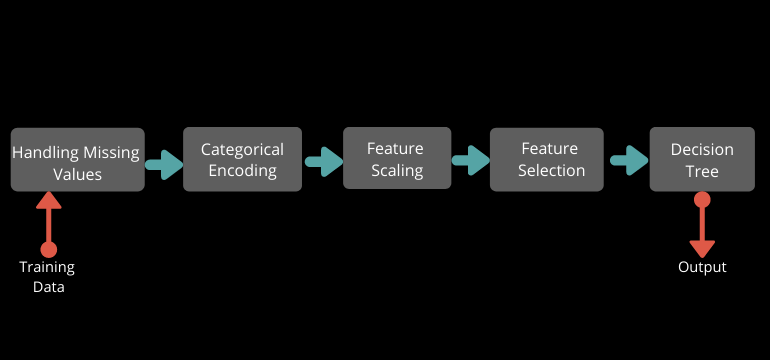
Putting this together with our Toyota cars dataset we can see how this improves (or not) our model
from sklearn.pipeline import Pipeline
from sklearn.feature_selection import SequentialFeatureSelector
from sklearn.feature_selection import chi2, SelectKBest
from sklearn import set_config
set_config(display='diagram')

# Reduce data frame to the top 1000 rows and select columns for regression analysis
toyota_df = load_data('ToyotaCorolla',nrows=1000,
            usecols=['Age_08_04', 'KM', 'Fuel_Type', 'HP', 'Met_Color', 'Automatic', 'CC', 'Doors', 'Quarterly_Tax', 'Weight', 'Price'])

outcome = 'Price'

num_columns = toyota_df.drop(columns=outcome).select_dtypes(include='number').columns
cat_columns = toyota_df.select_dtypes(exclude="number").columns

# Here we are going to apply two transforms to our numeric columns
# An imputer, to fill any gaps in our dataset with the median value
# And a scaler which we can use to ensure our data is standardized
numeric_transformer = Pipeline(
    steps=[("imputer", SimpleImputer(strategy="median")), ("scaler", StandardScaler())]
)

# For our categorical data, we'll use the OneHotEncoder
#  In essense this will dummy the columns for us
categorical_transformer = OneHotEncoder(handle_unknown="ignore")

column_transformer = ColumnTransformer(
    transformers=[
        ("num", numeric_transformer, num_columns),
        ("cat", categorical_transformer, cat_columns)])

toyota_reg = LinearRegression()

# Here we define the transformers to use and which columns to apply them too
pipeline = Pipeline([("col_transform",column_transformer)
            , ("feature_selection",SelectKBest())
            , ('regression_model',toyota_reg)])
pipeline
# And then, since we have our pipeline ready to go
toyota_X = toyota_df.drop(columns=outcome)
toyota_y = toyota_df[outcome]

toyota_X_train, toyota_X_test, toyota_y_train, toyota_y_test = train_test_split(toyota_X,toyota_y,train_size=0.8, random_state=123)
pipeline.fit(toyota_X_train,toyota_y_train)
toyota_y_pred = pipeline.predict(toyota_X_test)
regressionSummary(toyota_y_test, toyota_y_pred)
Other Available Prediction or Estimation Algorithms#
The same techniques apply when using any other prediction and estimation algorithm from the sklearn library. The data is prepared, split, fit and then predicted.
The following are a few other algorithm types (of which there are many deratives).
Support Vector Machines#
(from scikit-learning)
Support vector machines (SVMs) are a set of supervised learning methods used for classification, regression and outliers detection.
The advantages of support vector machines are:
Effective in high dimensional spaces.
Still effective in cases where number of dimensions is greater than the number of samples.
Uses a subset of training points in the decision function (called support vectors), so it is also memory efficient.
Versatile: different Kernel functions can be specified for the decision function. Common kernels are provided, but it is also possible to specify custom kernels.
The disadvantages of support vector machines include:
If the number of features is much greater than the number of samples, avoid over-fitting in choosing Kernel functions and regularization term is crucial.
SVMs do not directly provide probability estimates, these are calculated using an expensive five-fold cross-validation (see Scores and probabilities, below).
Nearest Neighbors#
(from scikit-learning)
In the same way that Nearest Neighbors for classification attempts to find the other observations which have the most similar predictors, Neighbors-based regression can be used in cases where the data labels are continuous rather than discrete variables. The label assigned to a query point is computed based on the mean of the labels of its nearest neighbors.
Decision Trees#
(from scikit-learning)
Decision Trees (DTs) are a non-parametric supervised learning method used for classification and regression. The goal is to create a model that predicts the value of a target variable by learning simple decision rules inferred from the data features. A tree can be seen as a piecewise constant approximation.
Some advantages of decision trees are:
Simple to understand and to interpret. Trees can be visualised.
Requires little data preparation. Other techniques often require data normalisation, dummy variables need to be created and blank values to be removed. Note however that this module does not support missing values.
The cost of using the tree (i.e., predicting data) is logarithmic in the number of data points used to train the tree.
Able to handle both numerical and categorical data. However scikit-learn implementation does not support categorical variables for now. Other techniques are usually specialised in analysing datasets that have only one type of * variable. See algorithms for more information.
Able to handle multi-output problems.
Uses a white box model. If a given situation is observable in a model, the explanation for the condition is easily explained by boolean logic. By contrast, in a black box model (e.g., in an artificial neural network), results may be more difficult to interpret.
Possible to validate a model using statistical tests. That makes it possible to account for the reliability of the model.
Performs well even if its assumptions are somewhat violated by the true model from which the data were generated.
The disadvantages of decision trees include:
Decision-tree learners can create over-complex trees that do not generalise the data well. This is called overfitting. Mechanisms such as pruning, setting the minimum number of samples required at a leaf node or setting the maximum depth of the tree are necessary to avoid this problem.
Decision trees can be unstable because small variations in the data might result in a completely different tree being generated. This problem is mitigated by using decision trees within an ensemble.
Predictions of decision trees are neither smooth nor continuous, but piecewise constant approximations as seen in the above figure. Therefore, they are not good at extrapolation.
The problem of learning an optimal decision tree is known to be NP-complete under several aspects of optimality and even for simple concepts. Consequently, practical decision-tree learning algorithms are based on heuristic algorithms such as the greedy algorithm where locally optimal decisions are made at each node. Such algorithms cannot guarantee to return the globally optimal decision tree. This can be mitigated by training multiple trees in an ensemble learner, where the features and samples are randomly sampled with replacement.
There are concepts that are hard to learn because decision trees do not express them easily, such as XOR, parity or multiplexer problems.
Decision tree learners create biased trees if some classes dominate. It is therefore recommended to balance the dataset prior to fitting with the decision tree.
Resources#
Other datasets suitable for regressions tasks#
Boston Housing]- predict the mean value of a homesSoftware Resale]- try to determine likely customer spend on softwareAirfare]- predict the airfare for new routesCancer Death Rates]- see if there is a set of predictors that can identifier higher death rate due to cancer